
Tankille.fi (part of kilpailuttaja.fi) is a community service for comparing the prices of gasoline, diesel, and other fuels. The prices are reported by users via the Tankille.fi mobile phone application. Popular petrol stations might receive several price updates per day, others sporadically. To increase the usefulness of the application, especially in the rural areas with infrequent reports, the application could provide an estimate of each station’s current price even in the absence of recent reports.
In the following, we examine the properties of the reported price data and then present steps to address the above challenge. Finally, we discuss the observed fuel pricing dynamics and the main obstacles imposed by the available data.
Data
The data contains 6 million user-submitted price reports for gasoline, diesel, and natural/bio gas (NG/BG) from nearly 2,200 stations between spring 2017 and fall 2025. Most fuel types appear in few price reports, and only 95E10, 98E5 and regular diesel exceed 20 % coverage. Due to high missigness, premium diesel, high-ethanol gasoline (15E85), biodiesel and NG/BG are excluded from the study.
Helsinki, Espoo and Vantaa account over 10% of all stations and generate over 20 % of all price reports. In general, share of reports correlates strongly with share of total population. ABC and Neste dominate with over 40 % combined share of stations. Together with ST1, Teboil and SEO they cover more than 80 % of all stations.
Reporting is highly concentrated and sparse: no station has reports for every day. Even the best stations miss a few days monthly, and 80 % of stations are observed on fewer than half of all days.
Methods
In this section we describe the preprocessing steps of the data, and present the hierarchical model for estimating fuel prices. The model has three layers, each targeting a specific subset of structure in the data; we describe these layers and their features in turn.
Data Preprocessing
We first remove price reports that (i) originated from users who never submit novel prices, (ii) do not have station metadata available (mainly older reports), (iii) are potentially fraudulent or (iv) belong to an “unreliable” user. A price report if fraudulent if the inter-report delay is less than legal top-speed travel times between the stations by car. An “unreliable” user is one who has ≥ 50 % of their price reports marked as fraudulent.
Next, we remove VAT and product taxes from prices to improve comparability across fuels. Data is then augmented with euro-denominated Brent crude end-of-day prices, the renewable fuel obligation (“Jakeluvelvoite”), the 12 primary components of Finnish monthly inflation (accounting for publication lags), and 1, 3, 6, and 12 month end-of-day EURIBOR rates.
Finally, reports are aggregated to daily mean prices by station and fuel type and temporal features (day of year, of month, and of week) are added using cyclic encoding.
National Trend Model
In the first stage we model and remove the trend from the daily national mean price per fuel type. Figure 1 shows national mean prices of 95E10, 98E5, and diesel in 2022. Russia’s invasion of Ukraine on 24 February 2022 triggered a sharp rise in prices, followed by a decline from mid-June, with a short lag in retail prices. Although the spread between 95E10 and 98E5 seems stable, it exhibits 3–6 month deviations of up to 10 % in either direction and permanent regime shifts.
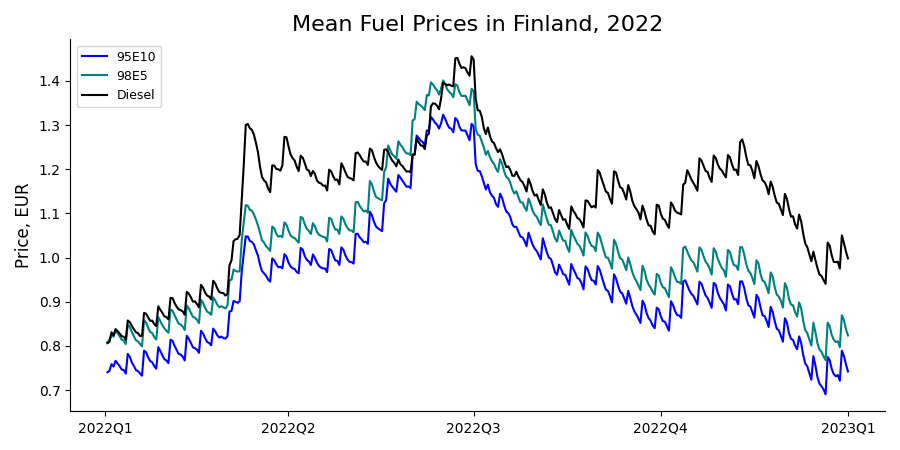
The daily sawtooth pattern in national prices reflects the “Wednesday phenomenon” (Edgeworth price cycles): prices spike midweek and then fall until early the next week. This pattern has been widely reported in Finland since at least 2021. In a September 25th 2023 blog post, the Finnish Competition and Consumer Authority attributed it to “silent collusion”, with a major chain acting as a price leader.
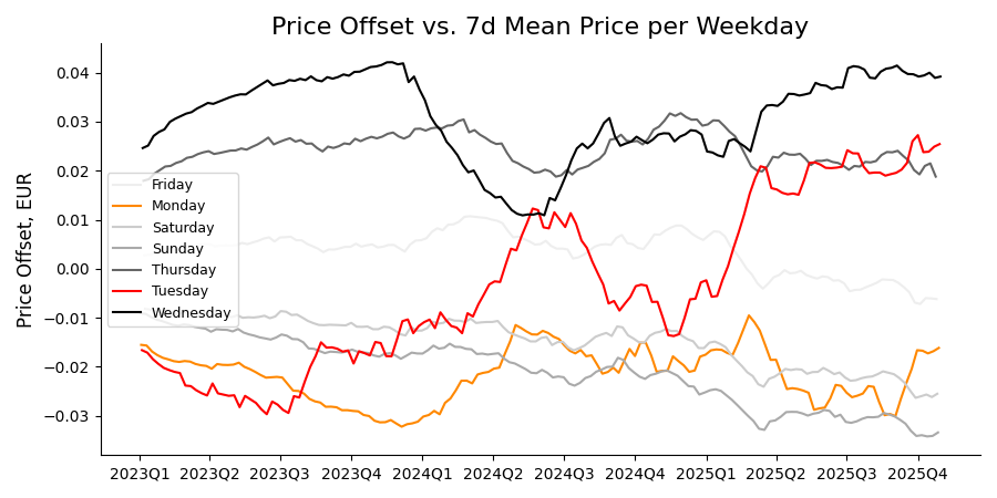
In a follow-up post on December 16th 2024, they note that the weekly peak has shifted and now occurs between Monday and Wednesday, while the cycle length remains about one week. They suggest St1 as a potential price leader. Figure 2 shows that Monday replaced Tuesday as the cheapest day in fall 2023, and in spring 2024 Tuesday had become as expensive as Wednesday. At the time of writing, Wednesday remains the most expensive day, with the spike typically beginning on Tuesday and often lasting through Thursday. Sunday is now the cheapest day, followed by Saturday.1
National Trend Model
We fit several models to the daily national mean price per fuel type using the features mentioned earlier: a baseline moving average, lasso and elastic net regression, support vector regression, gradient boosting regression, a feed-forward neural network, SARIMAX, and a Kalman filter. Hyperparameters are tuned with timeseries cross-validation. Out-of-sample accuracy is evaluated with MAD, MAE, MAPE, and RMSE.
With one month walk-forward evaluation, only the linear models and SVR outperform the baseline. SVR occasionally outperforms lasso but is much more expensive to train, making it unattractive. Lasso and elastic net perform similarly; lasso is faster and is therefore chosen as the national trend model.
Lagged prices, day of week and Brent price explain 99.9 % of the effect, 93 % of which solely from past national mean price. Brent price effect is 0.9 % for 95E10 and almost twice as strong for diesel and 98E5.
Chain-Level Pricing Model
Chain-level modeling uses price residuals of the national trend model: observed prices minus the fuel-specific national model predictions. Figure 3 clusters chains by annual mean price. Two chains, Keskinen and Kärkkäinen, are systematically cheaper than others. GT and independent stations have been getting almost exponentially more expensive since 2022. Seapoint price premium has been nearly 3x that of independent stations and has become steadily more expensive.
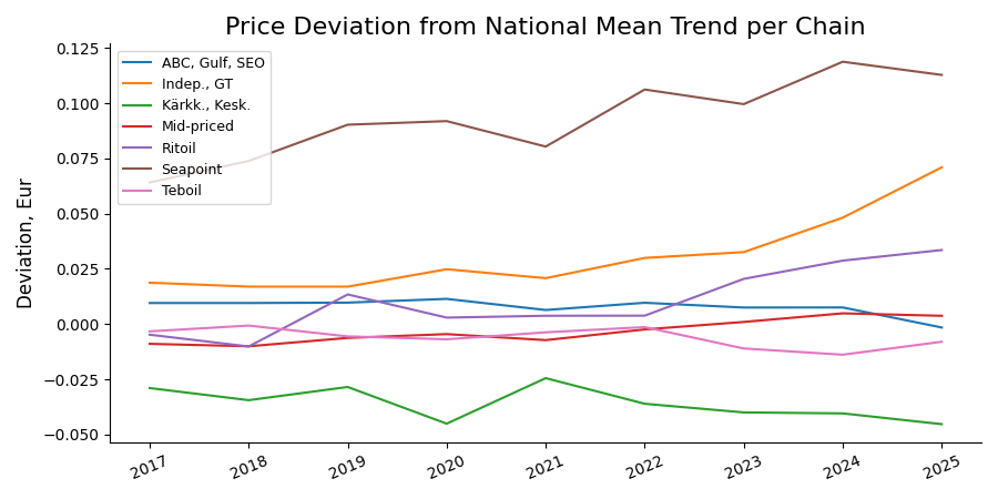
ABC (accompanied by Gulf and SEO) have had premium pricing but, from 2022 onward and especially in 2025, their prices have fallen toward the mid-priced group while Ritoil has moved into the more expensive group and continues to raise its level. Teboil, a mid-priced chain, has cut prices in 2022 markedly to offset its Russian ties; on November 21st 2025 Oy Teboil Ab filed for corporate restructuring.
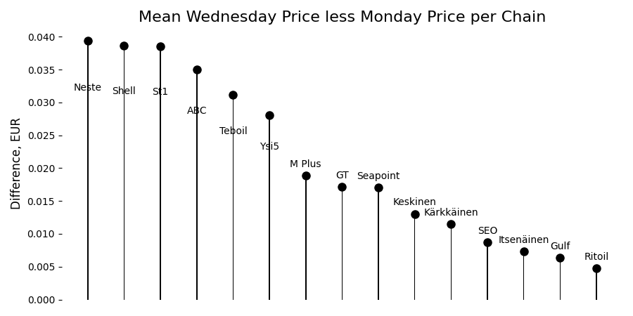
Figure 4 shows the midweek price spike by chain. Neste, ST1 and Shell raise prices by about 0.04 EUR from Monday to Wednesday.2 At the other extreme, SEO, independent stations, Gulf and Ritoil have a Monday-Wednesday difference below 0.01 EUR. As noted earlier, large chains dominate the reports, so their behavior is visible even in the unstratified national mean. The effect is not constant but has grown over time and is now stronger than ever.
For chain-level modeling we evaluate a moving-average baseline, lasso and elastic net regression, gradient boosting, Kalman filtering, and Prophet. We also evaluate two ensemble strategies: a stacking model, where a meta-learner uses covariates and base-model predictions to learn context-dependent weights, and an AutoML-style selector that trains all base models and chooses the best performer on a validation hold-out. In both cases the selected base learner(s) are finally refit on the full training period.
Lasso, elastic net, and GBR perform best on average and per-chain examination reveals regions where either lasso or GBR dominates. The AutoML ensemble exploits this pattern and is therefore chosen as the chain-level pricing model.
Station Specific Imputation Model
Station-level modeling uses price residuals of the chain-level model. Station-level data has two aspects: spatial and temporal. We first examine spatial variables that explain station-level price differences, then describe the temporal imputation model.
Spatial Effects on Station Prices
For spatial effects on per-station mean price we consider the station’s distances to its six nearest competitors, counts of competitors within radii from 100 m to 50 km, station density at postal-code level and all 100+ Paavo postal code statistic from Statistics Finland.
Lasso and GBR both find only negligible effects even with optimized subset of variables: while tiny fraction of stations might be affected by few variables enough to matter, over half of the 20 most influential variables have absolute effects below 0.0001 EUR for 75 % of stations. We therefore discard all spatial features and keep station prices unchanged rather than add modeling noise.
Temporal Effects on Station Prices
The final stage models intra- and inter-station correlations in the stationary per-station, per-fuel series. We hypothesize that a station’s current residual price depends on its own past prices and on current prices at other stations, each conditional on the others.
We form a matrix with timestamps as rows and station–fuel pairs as columns; each cell contains the residual price for that pair at that time. The matrix has nearly 1,400 rows, over 5,500 columns, and more than 70 % missing entries. Attempts to apply sparse variational Gaussian processes, linear coregionalization kernels, or a GPU-accelerated multivariate Kalman filter proved computationally infeasible. We therefore construct a rank-reduced Kalman filter that exploits cross-station correlations with modest memory and time requirements.
The rank-reduced filter works in two steps. First, missing values are imputed via iterative soft-thresholded SVD on standardized prices; then, we retain the top 1 % components and use them to define priors for a Kalman filter in the latent space. The filter predicts latent states which are mapped back to residual prices via the inverse of the first step. Our model improves on the baseline that assumes no per-station effects: in absolute terms, the imputation model’s MAE is in the range of 0.020-0.030 EUR, compared with 0.025-0.040 EUR for the baseline.
Conclusion
The study points to three main findings:
- fuel prices are overwhelmingly driven by their own past values. Simple linear models suffice on national and chain levels, and more complex methods add little.
- missingness is a binding constraint. Sparse and uneven reporting makes it difficult to study national or regional price leadership, or even to compare station-level pricing within a week. Data quality, rather than model sophistication, is thus the main limiter for causal or structural inference.
- we find no robust station-level spatial structure to exploit. This does not rule out station-level structure, but any such effects seem small relative to temporal dynamics and chain-level behavior.
Future Work
Future work concentrates on four directions:
- data cleaning removes a large share of reports; its assumptions and their impact on the composition of stations, fuels, regions, and years should be examined in detail.
- the hierarchical design should be contrasted with more unified models. A single joint model on a reduced, low-missingness subset would provide a baseline for what the hierarchy gives up.
- spatial structure deserves a more targeted analysis. Spatial effects may be more important in specific segments (urban/rural, coastal/inland, small/large chains). Finer-grained spatial data for urban areas, and additional constructs such as proximity to highways, city centers, major retailers, borders, fuel depots, or concentrations of company cars, may explain per-station pricing. Temporal patterns linked to holidays and to traffic intensity could be studied in the same spirit.
- missingness should be modeled explicitly. The relation between missingness and price level (or volatility) could bias inferences about cycles, chain differences, or volatility. Station-level imputation could be revisited with methods designed for irregular, incomplete time series such as GRU-D.
Acknowledgments
We gratefully acknowledge Kimmo Sivola of Energy Brokers Finland Oy (Kilpailuttaja.fi) for providing access to the data used in this study, and for useful feedback and domain expertise during the project.
Footnotes
[1] The national mean offset is below 0.05 EUR, whereas a single station can deviate 4–8 times more at a given instant. Because a station is rarely observed on both Monday and the following Wednesday, Monday prices are averaged nationally and compared with the national Wednesday mean, which masks much of the true within-station change.
[2] As with figure 2, using national mean prices masks much of the inter-station change.